Introductory Tutorial#
TimeseriesFlattener flattens timeseries. This is especially helpful if you have complicated and irregular time series but want to train simple models.
We explain terminology as needed in this tutorial. If you need a reference, see the docs.
Applying it consists of 3 steps:
Loading data (prediction times, predictor(s), and outcome(s))
Specifying how to flatten the data and
Flattening
The simplest case is adding one predictor and one outcome.
First, we’ll load the timestamps for every time we want to issue a prediction:
Loading data#
Loading prediction times#
Prediction times consist of two elements:
The entity id. This is the entity about which the prediction is issued. In medical contexts, this is frequently a patient.
The timestamp at which the prediction is to be issued.
from __future__ import annotations

from skimpy import skim
from timeseriesflattener.testing.load_synth_data import load_synth_prediction_times

df_prediction_times = load_synth_prediction_times()

skim(df_prediction_times)
df_prediction_times.sort(["entity_id"])
╭──────────────────────────────────────────────── skimpy summary ─────────────────────────────────────────────────╮
│          Data Summary                Data Types                                                                 │
│ ┏━━━━━━━━━━━━━━━━━━━┳━━━━━━━━┓ ┏━━━━━━━━━━━━━┳━━━━━━━┓                                                          │
│ ┃ dataframe         ┃ Values ┃ ┃ Column Type ┃ Count ┃                                                          │
│ ┡━━━━━━━━━━━━━━━━━━━╇━━━━━━━━┩ ┡━━━━━━━━━━━━━╇━━━━━━━┩                                                          │
│ │ Number of rows    │ 10000  │ │ int64       │ 1     │                                                          │
│ │ Number of columns │ 2      │ │ datetime64  │ 1     │                                                          │
│ └───────────────────┴────────┘ └─────────────┴───────┘                                                          │
│                                                     number                                                      │
│ ┏━━━━━━━━━━━━━━━━━━┳━━━━━━┳━━━━━━━━━┳━━━━━━━━━┳━━━━━━━━┳━━━━━━┳━━━━━━━━┳━━━━━━━━┳━━━━━━━━┳━━━━━━━━┳━━━━━━━━━━┓  │
│ ┃ column_name      ┃ NA   ┃ NA %    ┃ mean    ┃ sd     ┃ p0   ┃ p25    ┃ p50    ┃ p75    ┃ p100   ┃ hist     ┃  │
│ ┡━━━━━━━━━━━━━━━━━━╇━━━━━━╇━━━━━━━━━╇━━━━━━━━━╇━━━━━━━━╇━━━━━━╇━━━━━━━━╇━━━━━━━━╇━━━━━━━━╇━━━━━━━━╇━━━━━━━━━━┩  │
│ │ entity_id        │    0 │       0 │    4959 │   2886 │    0 │   2485 │   4922 │   7443 │   9999 │  ▇▇▇▇▇▇  │  │
│ └──────────────────┴──────┴─────────┴─────────┴────────┴──────┴────────┴────────┴────────┴────────┴──────────┘  │
│                                                    datetime                                                     │
│ ┏━━━━━━━━━━━━━━━━━━┳━━━━━━┳━━━━━━━━━┳━━━━━━━━━━━━━━━━━━━━━━━━━━━━┳━━━━━━━━━━━━━━━━━━━━━━━━━━━━┳━━━━━━━━━━━━━━┓  │
│ ┃ column_name      ┃ NA   ┃ NA %    ┃ first                      ┃ last                       ┃ frequency    ┃  │
│ ┡━━━━━━━━━━━━━━━━━━╇━━━━━━╇━━━━━━━━━╇━━━━━━━━━━━━━━━━━━━━━━━━━━━━╇━━━━━━━━━━━━━━━━━━━━━━━━━━━━╇━━━━━━━━━━━━━━┩  │
│ │ timestamp        │    0 │       0 │    1965-01-02 09:35:00     │    1969-12-31 21:42:00     │ None         │  │
│ └──────────────────┴──────┴─────────┴────────────────────────────┴────────────────────────────┴──────────────┘  │
╰────────────────────────────────────────────────────── End ──────────────────────────────────────────────────────╯
| entity_id | timestamp |
|---|---|
| i64 | datetime[μs] |
| 0 | 1969-01-11 09:55:00 |
| 1 | 1965-03-15 07:16:00 |
| 2 | 1969-09-13 23:18:00 |
| 3 | 1968-02-04 16:16:00 |
| 4 | 1965-01-28 12:33:00 |
| … | … |
| 9996 | 1965-01-30 17:19:00 |
| 9996 | 1965-07-18 17:12:00 |
| 9997 | 1967-06-08 07:52:00 |
| 9999 | 1965-07-19 14:59:00 |
| 9999 | 1968-02-07 22:24:00 |
Here, “entity_id” represents a patient ID and “timestamp” refers to the time when we want to issue a prediction. Note that each ID can have multiple prediction times.
Loading a temporal predictor#
Then, we’ll load the values for our temporal predictor. Temporal predictors are predictors that can have a different value at different timepoints.
from timeseriesflattener.testing.load_synth_data import load_synth_predictor_float

df_synth_predictors = load_synth_predictor_float()

skim(df_synth_predictors)
df_synth_predictors.sort(["entity_id"])
╭──────────────────────────────────────────────── skimpy summary ─────────────────────────────────────────────────╮
│          Data Summary                Data Types                                                                 │
│ ┏━━━━━━━━━━━━━━━━━━━┳━━━━━━━━┓ ┏━━━━━━━━━━━━━┳━━━━━━━┓                                                          │
│ ┃ dataframe         ┃ Values ┃ ┃ Column Type ┃ Count ┃                                                          │
│ ┡━━━━━━━━━━━━━━━━━━━╇━━━━━━━━┩ ┡━━━━━━━━━━━━━╇━━━━━━━┩                                                          │
│ │ Number of rows    │ 100000 │ │ int64       │ 1     │                                                          │
│ │ Number of columns │ 3      │ │ datetime64  │ 1     │                                                          │
│ └───────────────────┴────────┘ │ float64     │ 1     │                                                          │
│                                └─────────────┴───────┘                                                          │
│                                                     number                                                      │
│ ┏━━━━━━━━━━━━━━━━┳━━━━━┳━━━━━━━┳━━━━━━━━━┳━━━━━━━━━┳━━━━━━━━━━━━━┳━━━━━━━━┳━━━━━━━━┳━━━━━━━━┳━━━━━━━┳━━━━━━━━┓  │
│ ┃ column_name    ┃ NA  ┃ NA %  ┃ mean    ┃ sd      ┃ p0          ┃ p25    ┃ p50    ┃ p75    ┃ p100  ┃ hist   ┃  │
│ ┡━━━━━━━━━━━━━━━━╇━━━━━╇━━━━━━━╇━━━━━━━━━╇━━━━━━━━━╇━━━━━━━━━━━━━╇━━━━━━━━╇━━━━━━━━╇━━━━━━━━╇━━━━━━━╇━━━━━━━━┩  │
│ │ entity_id      │   0 │     0 │    4994 │    2887 │           0 │   2486 │   4996 │   7487 │  9999 │ ▇▇▇▇▇▇ │  │
│ │ value          │   0 │     0 │   4.983 │   2.885 │   0.0001514 │  2.483 │  4.975 │  7.486 │    10 │ ▇▇▇▇▇▇ │  │
│ └────────────────┴─────┴───────┴─────────┴─────────┴─────────────┴────────┴────────┴────────┴───────┴────────┘  │
│                                                    datetime                                                     │
│ ┏━━━━━━━━━━━━━━━━━━┳━━━━━━┳━━━━━━━━━┳━━━━━━━━━━━━━━━━━━━━━━━━━━━━┳━━━━━━━━━━━━━━━━━━━━━━━━━━━━┳━━━━━━━━━━━━━━┓  │
│ ┃ column_name      ┃ NA   ┃ NA %    ┃ first                      ┃ last                       ┃ frequency    ┃  │
│ ┡━━━━━━━━━━━━━━━━━━╇━━━━━━╇━━━━━━━━━╇━━━━━━━━━━━━━━━━━━━━━━━━━━━━╇━━━━━━━━━━━━━━━━━━━━━━━━━━━━╇━━━━━━━━━━━━━━┩  │
│ │ timestamp        │    0 │       0 │    1965-01-02 00:01:00     │    1969-12-31 23:37:00     │ None         │  │
│ └──────────────────┴──────┴─────────┴────────────────────────────┴────────────────────────────┴──────────────┘  │
╰────────────────────────────────────────────────────── End ──────────────────────────────────────────────────────╯
| entity_id | timestamp | value |
|---|---|---|
| i64 | datetime[μs] | f64 |
| 0 | 1967-06-12 14:06:00 | 0.174793 |
| 0 | 1968-04-15 01:45:00 | 3.072293 |
| 0 | 1968-12-09 05:42:00 | 1.315754 |
| 0 | 1969-06-20 18:07:00 | 2.812481 |
| 0 | 1967-11-26 01:59:00 | 2.981185 |
| … | … | … |
| 9999 | 1968-08-19 10:15:00 | 0.671907 |
| 9999 | 1966-01-03 22:34:00 | 4.158796 |
| 9999 | 1966-06-27 10:55:00 | 4.414455 |
| 9999 | 1968-04-02 12:58:00 | 1.552491 |
| 9999 | 1969-06-24 07:19:00 | 4.501553 |
Once again, note that there can be multiple values for each ID.
Loading a static predictor#
Frequently, you’ll have one or more static predictors describing each entity. In this case, an entity is a patient, and an example of a static outcome could be their sex. It doesn’t change over time (it’s static), but can be used as a predictor for each prediction time. Let’s load it in!
from timeseriesflattener.testing.load_synth_data import load_synth_sex

df_synth_sex = load_synth_sex()

skim(df_synth_sex)
df_synth_sex
╭──────────────────────────────────────────────── skimpy summary ─────────────────────────────────────────────────╮
│          Data Summary                Data Types                                                                 │
│ ┏━━━━━━━━━━━━━━━━━━━┳━━━━━━━━┓ ┏━━━━━━━━━━━━━┳━━━━━━━┓                                                          │
│ ┃ dataframe         ┃ Values ┃ ┃ Column Type ┃ Count ┃                                                          │
│ ┡━━━━━━━━━━━━━━━━━━━╇━━━━━━━━┩ ┡━━━━━━━━━━━━━╇━━━━━━━┩                                                          │
│ │ Number of rows    │ 9999   │ │ int64       │ 2     │                                                          │
│ │ Number of columns │ 2      │ └─────────────┴───────┘                                                          │
│ └───────────────────┴────────┘                                                                                  │
│                                                     number                                                      │
│ ┏━━━━━━━━━━━━━━━━━━┳━━━━━━┳━━━━━━━━┳━━━━━━━━━━━┳━━━━━━━━┳━━━━━━┳━━━━━━━━┳━━━━━━━━┳━━━━━━━━┳━━━━━━━━┳━━━━━━━━━┓  │
│ ┃ column_name      ┃ NA   ┃ NA %   ┃ mean      ┃ sd     ┃ p0   ┃ p25    ┃ p50    ┃ p75    ┃ p100   ┃ hist    ┃  │
│ ┡━━━━━━━━━━━━━━━━━━╇━━━━━━╇━━━━━━━━╇━━━━━━━━━━━╇━━━━━━━━╇━━━━━━╇━━━━━━━━╇━━━━━━━━╇━━━━━━━━╇━━━━━━━━╇━━━━━━━━━┩  │
│ │ entity_id        │    0 │      0 │      4999 │   2887 │    0 │   2500 │   4999 │   7500 │   9999 │ ▇▇▇▇▇▇  │  │
│ │ female           │    0 │      0 │    0.4984 │    0.5 │    0 │      0 │      0 │      1 │      1 │ ▇    ▇  │  │
│ └──────────────────┴──────┴────────┴───────────┴────────┴──────┴────────┴────────┴────────┴────────┴─────────┘  │
╰────────────────────────────────────────────────────── End ──────────────────────────────────────────────────────╯
| entity_id | female |
|---|---|
| i64 | i64 |
| 0 | 0 |
| 1 | 1 |
| 2 | 1 |
| 3 | 1 |
| 4 | 0 |
| … | … |
| 9995 | 0 |
| 9996 | 0 |
| 9997 | 1 |
| 9998 | 1 |
| 9999 | 0 |
As the predictor is static, there should only be a single value for each ID in this dataframe.
Loading a temporal outcome#
And, lastly, our outcome values. We’ve chosen a binary outcome and only stored values for the timestamps that experience the outcome. From these, we can infer patients that do not experience the outcome, since they do not have a timestamp. We handle this by setting a fallback of 0 - more on that in the following section.
from timeseriesflattener.testing.load_synth_data import load_synth_outcome

df_synth_outcome = load_synth_outcome()

skim(df_synth_outcome)
df_synth_outcome
╭──────────────────────────────────────────────── skimpy summary ─────────────────────────────────────────────────╮
│          Data Summary                Data Types                                                                 │
│ ┏━━━━━━━━━━━━━━━━━━━┳━━━━━━━━┓ ┏━━━━━━━━━━━━━┳━━━━━━━┓                                                          │
│ ┃ dataframe         ┃ Values ┃ ┃ Column Type ┃ Count ┃                                                          │
│ ┡━━━━━━━━━━━━━━━━━━━╇━━━━━━━━┩ ┡━━━━━━━━━━━━━╇━━━━━━━┩                                                          │
│ │ Number of rows    │ 3103   │ │ int64       │ 2     │                                                          │
│ │ Number of columns │ 3      │ │ datetime64  │ 1     │                                                          │
│ └───────────────────┴────────┘ └─────────────┴───────┘                                                          │
│                                                     number                                                      │
│ ┏━━━━━━━━━━━━━━━━━━┳━━━━━━┳━━━━━━━━━┳━━━━━━━━━┳━━━━━━━━┳━━━━━━┳━━━━━━━━┳━━━━━━━━┳━━━━━━━━┳━━━━━━━━┳━━━━━━━━━━┓  │
│ ┃ column_name      ┃ NA   ┃ NA %    ┃ mean    ┃ sd     ┃ p0   ┃ p25    ┃ p50    ┃ p75    ┃ p100   ┃ hist     ┃  │
│ ┡━━━━━━━━━━━━━━━━━━╇━━━━━━╇━━━━━━━━━╇━━━━━━━━━╇━━━━━━━━╇━━━━━━╇━━━━━━━━╇━━━━━━━━╇━━━━━━━━╇━━━━━━━━╇━━━━━━━━━━┩  │
│ │ entity_id        │    0 │       0 │    5032 │   2900 │    4 │   2499 │   5109 │   7555 │   9992 │  ▇▇▇▇▇▇  │  │
│ │ value            │    0 │       0 │       1 │      0 │    1 │      1 │      1 │      1 │      1 │      ▇   │  │
│ └──────────────────┴──────┴─────────┴─────────┴────────┴──────┴────────┴────────┴────────┴────────┴──────────┘  │
│                                                    datetime                                                     │
│ ┏━━━━━━━━━━━━━━━━━━┳━━━━━━┳━━━━━━━━━┳━━━━━━━━━━━━━━━━━━━━━━━━━━━━┳━━━━━━━━━━━━━━━━━━━━━━━━━━━━┳━━━━━━━━━━━━━━┓  │
│ ┃ column_name      ┃ NA   ┃ NA %    ┃ first                      ┃ last                       ┃ frequency    ┃  │
│ ┡━━━━━━━━━━━━━━━━━━╇━━━━━━╇━━━━━━━━━╇━━━━━━━━━━━━━━━━━━━━━━━━━━━━╇━━━━━━━━━━━━━━━━━━━━━━━━━━━━╇━━━━━━━━━━━━━━┩  │
│ │ timestamp        │    0 │       0 │    1965-01-04 07:50:00     │    1969-12-31 10:15:00     │ None         │  │
│ └──────────────────┴──────┴─────────┴────────────────────────────┴────────────────────────────┴──────────────┘  │
╰────────────────────────────────────────────────────── End ──────────────────────────────────────────────────────╯
| entity_id | timestamp | value |
|---|---|---|
| i64 | datetime[μs] | i64 |
| 9263 | 1966-10-05 17:03:00 | 1 |
| 5642 | 1967-09-25 17:17:00 | 1 |
| 667 | 1967-12-22 07:20:00 | 1 |
| 834 | 1969-04-06 11:46:00 | 1 |
| 2906 | 1965-08-28 22:16:00 | 1 |
| … | … | … |
| 759 | 1969-05-25 19:49:00 | 1 |
| 7124 | 1967-08-21 16:15:00 | 1 |
| 6984 | 1965-01-20 17:42:00 | 1 |
| 9759 | 1965-02-11 12:48:00 | 1 |
| 5844 | 1969-05-07 23:50:00 | 1 |
This dataframe should contain at most 1 row per ID, which is the first time they experience the outcome.
We now have 4 dataframes loaded: df_prediction_times, df_synth_predictors, df_synth_sex and df_synth_outcome.
Specifying how to flatten the data#
We’ll have to specify how to flatten predictors and outcomes. To do this, we use the feature specification objects as “recipes” for each column in our finished dataframe. Firstly, we’ll specify the outcome specification.
Temporal outcome specification#
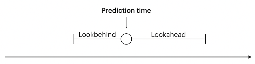
The main decision to make for outcomes is the size of the lookahead window. It determines how far into the future from a given prediction time to look for outcome values. A prediction time indicates at which point the model issues a prediction, and is used as a reference for the lookahead.

We want labels for prediction times to be 0 if the outcome never occurs, or if the outcome happens outside the lookahead window. Labels should only be 1 if the outcome occurs inside the lookahead window. Let’s specify this in code.
import datetime as dt

import pandas as pd
from timeseriesflattener import BooleanOutcomeSpec, TimestampValueFrame, ValueFrame
from timeseriesflattener.aggregators import MaxAggregator

test_df = pd.DataFrame({"entity_id": [0], "timestamp": [pd.Timestamp("2020-01-01")]})

outcome_spec = BooleanOutcomeSpec.from_primitives(
    df=test_df,
    entity_id_col_name="entity_id",
    value_timestamp_col_name="timestamp",
    lookahead_days=[365],
    aggregators=["max"],
    column_prefix="outc",
)

# Alternatively, if you prefer types
outcome_spec = BooleanOutcomeSpec(
    init_frame=TimestampValueFrame(
        entity_id_col_name="entity_id", init_df=test_df, value_timestamp_col_name="timestamp"
    ),
    lookahead_distances=[dt.timedelta(days=365)],
    aggregators=[MaxAggregator()],
    output_name="outcome",
    column_prefix="outc",
)
Since our outcome is binary, we want each prediction time to be labeled with 0 for the outcome if none is present within lookahead days. To do this, we use the fallback argument, which specifies the default value to use if none are found in values_df within lookahead. For the BooleanOutcomeSpec, this is hardcoded to 0.
Your use case determines how you want to handle multiple outcome values within lookahead days. In this case, we decide that any prediction time with at least one outcome (a timestamp in the loaded outcome data with a corresponding value of 1) within the specified lookahead days is “positive”. I.e., if there is both a 0 and a 1 within lookahead days, the prediction time should be labeled with a 1. We set aggregators = [MaxAggregator()] to accomplish this.
Here, we specifiy that we want to look 365 days forward from the prediction time to search for outcomes. If we wanted to require a certain period of time from the prediction time before we look for outcome values, we can specify lookahead as an interval of (min_days, max_days) as a tuple instead.
Lastly, we specify a name of the outcome which’ll be used when generating its column.
Temporal predictor specification#
Specifying a predictor is almost entirely identical to specifying an outcome. The only exception is that it looks a given number of days into the past from each prediction time instead of ahead.
import numpy as np
from timeseriesflattener import PredictorSpec, StaticSpec
from timeseriesflattener.aggregators import MeanAggregator

temporal_predictor_spec = PredictorSpec.from_primitives(
    df=df_synth_predictors.rename({"value": "value_1"}),
    entity_id_col_name="entity_id",
    value_timestamp_col_name="timestamp",
    aggregators=["mean"],
    column_prefix="pred",
    fallback=np.nan,
    lookbehind_days=[730],
)

# Alternatively, if you prefer types

temporal_predictor_spec = PredictorSpec(
    value_frame=ValueFrame(
        entity_id_col_name="entity_id",
        init_df=df_synth_predictors.rename({"value": "value_1"}),
        value_timestamp_col_name="timestamp",
    ),
    aggregators=[MeanAggregator()],
    column_prefix="pred",
    fallback=np.nan,
    lookbehind_distances=[dt.timedelta(days=730)],
)

Values within the lookbehind window are aggregated using aggregators, for example the mean as shown in this example, or max/min etc.
Note that we rename the value column to value_1. The value column’s name determines the name of the output column after aggregation. To avoid multiple output columns with the same name, all input value columns must have unique names.
Temporal predictors can also be specified to look for values within a certain time range from the prediction time, similar to outcome specifications. For instance, you might want to create multiple predictors, where one looks for values within (0, 30) days, and another within (31, 182) days.
This can easily be specified by passing a tuple[min_days, max_days] to the lookbehind_days parameter.
temporal_interval_predictor_spec = PredictorSpec.from_primitives(
    df=df_synth_predictors.rename({"value": "value_2"}),
    entity_id_col_name="entity_id",
    value_timestamp_col_name="timestamp",
    aggregators=["mean"],
    column_prefix="pred",
    fallback=np.nan,
    lookbehind_days=[(10, 365)],
)

# Alternatively, if you prefer types
temporal_interval_predictor_spec = PredictorSpec(
    value_frame=ValueFrame(
        entity_id_col_name="entity_id",
        init_df=df_synth_predictors.rename({"value": "value_2"}),
        value_timestamp_col_name="timestamp",
    ),
    aggregators=[MeanAggregator()],
    column_prefix="pred",
    fallback=np.nan,
    lookbehind_distances=[(dt.timedelta(days=10), dt.timedelta(days=365))],
)
Static predictor specification#
Static features should be specified using StaticSpec as they are handled slightly differently. As in the previous specifications, we provide a values_df containing the values and we set the feature name. However, now we also add a prefix. By default, PredictorSpec prefixes columns with “pred” and OutcomeSpec prefixes columns with “outc” to make filtering easy.
As StaticSpec can be used for both generating predictors and outcomes, we manually set the prefix to be “pred”, as sex is used as predictor in this case.
from timeseriesflattener import StaticFrame

sex_predictor_spec = StaticSpec.from_primitives(
    df=df_synth_sex, entity_id_col_name="entity_id", column_prefix="pred", fallback=np.nan
)

# Alternatively, if you prefer types
sex_predictor_spec = StaticSpec(
    value_frame=StaticFrame(init_df=df_synth_sex), column_prefix="pred", fallback=np.nan
)

df_synth_sex
| entity_id | female |
|---|---|
| i64 | i64 |
| 0 | 0 |
| 1 | 1 |
| 2 | 1 |
| 3 | 1 |
| 4 | 0 |
| … | … |
| 9995 | 0 |
| 9996 | 0 |
| 9997 | 1 |
| 9998 | 1 |
| 9999 | 0 |
Note that we don’t need to specify which columns to aggregate. Timeseriesflattener aggregates all columns that are not entity_id_col_name or value_timestamp_col_name and uses the name(s) of the column(s) for the output.
Now we’re ready to flatten our dataset!
Flattening#
Flattening is as easy as instantiating the TimeseriesFlattener class with the prediction times df along with dataset specific metadata and calling the add_* functions. n_workers can be set to parallelize operations across multiple cores.
from timeseriesflattener import Flattener, PredictionTimeFrame

flattener = Flattener(
    predictiontime_frame=PredictionTimeFrame(
        init_df=df_prediction_times, entity_id_col_name="entity_id", timestamp_col_name="timestamp"
    )
)
df = flattener.aggregate_timeseries(
    specs=[
        sex_predictor_spec,
        temporal_predictor_spec,
        temporal_interval_predictor_spec,
        outcome_spec,
    ]
).df

skim(df)

list(df.columns)
Processing spec: ['female']
Processing spec: ['value_1']
Processing spec: ['value_2']
Processing spec: ['outcome']
╭──────────────────────────────────────────────── skimpy summary ─────────────────────────────────────────────────╮
│          Data Summary                Data Types                                                                 │
│ ┏━━━━━━━━━━━━━━━━━━━┳━━━━━━━━┓ ┏━━━━━━━━━━━━━┳━━━━━━━┓                                                          │
│ ┃ dataframe         ┃ Values ┃ ┃ Column Type ┃ Count ┃                                                          │
│ ┡━━━━━━━━━━━━━━━━━━━╇━━━━━━━━┩ ┡━━━━━━━━━━━━━╇━━━━━━━┩                                                          │
│ │ Number of rows    │ 10000  │ │ int64       │ 3     │                                                          │
│ │ Number of columns │ 7      │ │ float64     │ 2     │                                                          │
│ └───────────────────┴────────┘ │ datetime64  │ 1     │                                                          │
│                                │ string      │ 1     │                                                          │
│                                └─────────────┴───────┘                                                          │
│                                                     number                                                      │
│ ┏━━━━━━━━━━━━━━━━━━━━━━━┳━━━━━━┳━━━━━━━┳━━━━━━━━┳━━━━━━━┳━━━━━━━━━━━┳━━━━━━━┳━━━━━━━┳━━━━━━━┳━━━━━━━┳━━━━━━━━┓  │
│ ┃ column_name           ┃ NA   ┃ NA %  ┃ mean   ┃ sd    ┃ p0        ┃ p25   ┃ p50   ┃ p75   ┃ p100  ┃ hist   ┃  │
│ ┡━━━━━━━━━━━━━━━━━━━━━━━╇━━━━━━╇━━━━━━━╇━━━━━━━━╇━━━━━━━╇━━━━━━━━━━━╇━━━━━━━╇━━━━━━━╇━━━━━━━╇━━━━━━━╇━━━━━━━━┩  │
│ │ entity_id             │    0 │     0 │   4959 │  2886 │         0 │  2485 │  4922 │  7443 │  9999 │ ▇▇▇▇▇▇ │  │
│ │ pred_female_fallback_ │    0 │     0 │ 0.4931 │   0.5 │         0 │     0 │     0 │     1 │     1 │ ▇    ▇ │  │
│ │ nan                   │      │       │        │       │           │       │       │       │       │        │  │
│ │ pred_value_1_within_0 │ 1072 │ 10.72 │   5.01 │ 1.842 │   0.01491 │ 3.851 │ 5.023 │ 6.178 │ 9.946 │ ▁▃▇▇▃▁ │  │
│ │ _to_730_days_mean_fal │      │       │        │       │           │       │       │       │       │        │  │
│ │ lback_nan             │      │       │        │       │           │       │       │       │       │        │  │
│ │ pred_value_2_within_1 │ 2060 │  20.6 │  5.008 │ 2.222 │ 0.0003901 │  3.52 │ 5.014 │  6.56 │ 9.997 │ ▂▅▇▇▅▂ │  │
│ │ 0_to_365_days_mean_fa │      │       │        │       │           │       │       │       │       │        │  │
│ │ llback_nan            │      │       │        │       │           │       │       │       │       │        │  │
│ │ outc_outcome_within_0 │    0 │     0 │      0 │     0 │         0 │     0 │     0 │     0 │     0 │     ▇  │  │
│ │ _to_365_days_max_fall │      │       │        │       │           │       │       │       │       │        │  │
│ │ back_0                │      │       │        │       │           │       │       │       │       │        │  │
│ └───────────────────────┴──────┴───────┴────────┴───────┴───────────┴───────┴───────┴───────┴───────┴────────┘  │
│                                                    datetime                                                     │
│ ┏━━━━━━━━━━━━━━━━━━┳━━━━━━┳━━━━━━━━━┳━━━━━━━━━━━━━━━━━━━━━━━━━━━━┳━━━━━━━━━━━━━━━━━━━━━━━━━━━━┳━━━━━━━━━━━━━━┓  │
│ ┃ column_name      ┃ NA   ┃ NA %    ┃ first                      ┃ last                       ┃ frequency    ┃  │
│ ┡━━━━━━━━━━━━━━━━━━╇━━━━━━╇━━━━━━━━━╇━━━━━━━━━━━━━━━━━━━━━━━━━━━━╇━━━━━━━━━━━━━━━━━━━━━━━━━━━━╇━━━━━━━━━━━━━━┩  │
│ │ timestamp        │    0 │       0 │    1965-01-02 09:35:00     │    1969-12-31 21:42:00     │ None         │  │
│ └──────────────────┴──────┴─────────┴────────────────────────────┴────────────────────────────┴──────────────┘  │
│                                                     string                                                      │
│ ┏━━━━━━━━━━━━━━━━━━━━━━━━━━━━━━━━━━━━━━━┳━━━━━━━┳━━━━━━━━━━━┳━━━━━━━━━━━━━━━━━━━━━━━━━━┳━━━━━━━━━━━━━━━━━━━━━┓  │
│ ┃ column_name                           ┃ NA    ┃ NA %      ┃ words per row            ┃ total words         ┃  │
│ ┡━━━━━━━━━━━━━━━━━━━━━━━━━━━━━━━━━━━━━━━╇━━━━━━━╇━━━━━━━━━━━╇━━━━━━━━━━━━━━━━━━━━━━━━━━╇━━━━━━━━━━━━━━━━━━━━━┩  │
│ │ prediction_time_uuid                  │     0 │         0 │                        2 │               20000 │  │
│ └───────────────────────────────────────┴───────┴───────────┴──────────────────────────┴─────────────────────┘  │
╰────────────────────────────────────────────────────── End ──────────────────────────────────────────────────────╯
['entity_id',
 'timestamp',
 'prediction_time_uuid',
 'pred_female_fallback_nan',
 'pred_value_1_within_0_to_730_days_mean_fallback_nan',
 'pred_value_2_within_10_to_365_days_mean_fallback_nan',
 'outc_outcome_within_0_to_365_days_max_fallback_0']
# For displayability, shorten col names
shortened_pred = "predX"
shortened_predinterval = "predX_30_to_90"
shortened_outcome = "outc_Y"

display_df = df.rename(
    {
        "pred_value_1_within_0_to_730_days_mean_fallback_nan": shortened_pred,
        "pred_value_2_within_10_to_365_days_mean_fallback_nan": shortened_predinterval,
        "outc_outcome_within_0_to_365_days_max_fallback_0": shortened_outcome,
    }
)
display_df
| entity_id | timestamp | prediction_time_uuid | pred_female_fallback_nan | predX | predX_30_to_90 | outc_Y |
|---|---|---|---|---|---|---|
| i64 | datetime[μs] | str | i64 | f64 | f64 | i32 |
| 9852 | 1965-01-02 09:35:00 | "9852-1965-01-02 09:35:00.00000… | 1 | NaN | NaN | 0 |
| 1467 | 1965-01-02 10:05:00 | "1467-1965-01-02 10:05:00.00000… | 0 | NaN | NaN | 0 |
| 1125 | 1965-01-02 12:55:00 | "1125-1965-01-02 12:55:00.00000… | 0 | NaN | NaN | 0 |
| 649 | 1965-01-02 14:01:00 | "649-1965-01-02 14:01:00.000000" | 0 | NaN | NaN | 0 |
| 2070 | 1965-01-03 08:01:00 | "2070-1965-01-03 08:01:00.00000… | 1 | NaN | NaN | 0 |
| … | … | … | … | … | … | … |
| 334 | 1969-12-31 16:32:00 | "334-1969-12-31 16:32:00.000000" | 1 | 7.252526 | NaN | 0 |
| 3363 | 1969-12-31 17:52:00 | "3363-1969-12-31 17:52:00.00000… | 1 | 3.679667 | 2.409664 | 0 |
| 7929 | 1969-12-31 18:22:00 | "7929-1969-12-31 18:22:00.00000… | 0 | 4.943585 | 7.475979 | 0 |
| 6002 | 1969-12-31 20:07:00 | "6002-1969-12-31 20:07:00.00000… | 1 | 5.593583 | 7.076598 | 0 |
| 864 | 1969-12-31 21:42:00 | "864-1969-12-31 21:42:00.000000" | 1 | 5.520416 | NaN | 0 |
And there we go! A dataframe ready for classification, containing:
The citizen IDs
Timestamps for each prediction time
A unique identifier for each prediciton-time
Our predictor columns, prefixed with
pred_andOur outcome columns, prefixed with
outc_